Spin Squeezing
Quantum systems are inherently difficult to measure precisely, due to the variance in every measurement as codified by the Heisenberg uncertainty principle. In this post we look at the method of spin squeezing, which is a way to increase the precision of measurement of a specific quantity by using entanglement.
The Setup
Let’s consider a quantum system of \(N\) spin-\(1/2\) particles, initially prepared in an non-entangled state. These could be electrons, but in this post, we will just refer to them as particles.
In this scenario, we take each particle to be prepared in a coherent superposition of spin-up \(|\uparrow\rangle\) and spin-down \(|\downarrow\rangle\):
\begin{equation} \left|\psi\right\rangle = \cos\left(\frac{\theta}{2}\right)|\uparrow\rangle + e^{i\phi}\sin\left(\frac{\theta}{2}\right)|\downarrow\rangle \label{eq:1} \end{equation}
If we measure the spin vector, \(\vec{S}_i\), of the \(i^{th}\) particle, quantum mechanics predicts that the expected value will be:
\[ \left\langle \vec{S}_i \right\rangle = \frac{1}{2} \left(\sin(\theta)\cos(\phi)\hat{x} + \sin(\theta)\sin(\phi)\hat{y} + \cos(\theta)\hat{z} \right) \]
Now, the composite system of the \(N\) spins can be described as the product state of all the single states:
\[ \left|\Psi\right\rangle = \bigotimes^N_i \left|\psi\right\rangle_i \]
This state we will call the coherent spin state. If we calculate the expected value of the total spin vector of this state:
\[ \vec{S} = \sum_{i=1}^N \vec{S}_i \]
The result is just \(N\) times the single particle value:
\[ \left\langle \vec{S} \right\rangle = \frac{N}{2}\sin{\theta}\cos{\phi}\hat{x} + \frac{N}{2}\sin{\theta}\sin{\phi}\hat{y} + \frac{N}{2}\cos{\theta}\hat{z} \]
The direction this vector points in is referred to as the mean spin direction (or MSD), since it is the average (or mean) direction of all the constituent particles' spin vectors.
We can form a unit vector \(\hat{n}_\perp\) which is perpendicular to the MSD such that \(\langle \vec{S} \rangle \cdot \hat{n}_\perp = \left\langle \vec{S}\cdot\hat{n}_{\perp} \right\rangle = 0\) .
Now although the average value of \(\vec{S}\cdot\hat{n}_{\perp}\) is zero, the variance of this quantity will be positive:
\[ \sigma^2_{\vec{S}\cdot\hat{n}_{\perp}} \equiv \left\langle \left(\vec{S}\cdot\hat{n}_{\perp}\right)^2 \right\rangle - \left\langle \vec{S}\cdot\hat{n}_{\perp} \right\rangle^2 = \left\langle \left(\vec{S}\cdot\hat{n}_{\perp}\right)^2 \right\rangle > 0 \]
Also, since we are in 3D, we can form another unit vector \(\hat{m}_\perp\) that is perpendicular to \(\hat{n}_\perp\) and the MSD.
In the initial state of the system, the variances are equal:
\[ \sigma^2_{\vec{S}\cdot\hat{m}_{\perp}} = \sigma^2_{\vec{S}\cdot\hat{n}_{\perp}} \]
In fact, since this is true for arbitrary \(\hat{n}_\perp\) and \(\hat{m}_\perp\) (as long as they are perpendicular to the MSD), the variance of \(\vec{S}\) is isotropic in this state. In other words, if we parameterize \(\hat{n}_\perp\) in terms of an angle \(\varphi \in [0, 2\pi)\):
\[ \hat{n}_\perp = \hat{\eta}\sin{\varphi} + \hat{\xi}\cos{\varphi} \]
Then the variance of \(S_{\varphi}\), where
\[ S_{\varphi} = \vec{S}\cdot\hat{n}_\perp = S_\eta\sin\varphi + S_\xi\cos\varphi \]
is constant as we sweep \(\hat{n}_{\perp}\) around the circle:
\[ \sigma^2_{S_\varphi} = \text{constant for all } \varphi \]
Now the imprecision in our measurement is directly proportional to \(\sigma^2_{S_{\phi}}\). So, if we seek to precisely measure the spin vector of this system, we had better find a way to reduce it. There’s just one problem.
Since this is a quantum system, the variance of our measurements cannot be decreased to zero. This is known as the Heisenberg uncertainty principle, which in this context reads:
\[ \sigma^2_{\vec{S}\cdot\hat{n}_{\perp}}\sigma^2_{\vec{S}\cdot\hat{m}_{\perp}} \geq \frac{1}{4} \left|\left\langle \vec{S}\cdot (\hat{n}_\perp\times \hat{m}_\perp)\right\rangle\right|^2 \]
This inequality describes a certain trade-off, since the smaller we make \(\sigma^2_{\vec{S}\cdot\hat{n}_\perp}\), the larger \(\sigma^2_{\vec{S}\cdot\hat{m}_\perp}\) becomes, and vice-versa. In other words, if we try to decrease the variance in one direction, we will increase the variance in the perpendicular direction. This kind of effect motivates the name spin squeezing.
Introducing Squeezing
Now that we know what spin squeezing is, how would one actually go about doing it?
There are a couple of ways to implement it, but they all require generating entanglement between the particles. One way to do this is called the one-axis twisting method in the literature. With this method, the individual quantum states \(|\psi\rangle\) are prepared as in \eqref{eq:1} with \(\theta = \frac{\pi}{2}\), \(\phi=0\). Then we couple the \(z\) -component of each particle’s spin vector with the \(z\) -component of every other particle’s spin vector. The Hamiltonian for this interaction is:
\[ H = \sum_{i\neq j} S_i^z S_j^z \]
The spin squeezing operator in this context is defined as:
\[ U(t) = \exp\left(-\frac{i}{2}t \sum_{i \neq j}^N S^z_i S^z_j\right) \]
We apply it to our initial state \(|\Psi\rangle\) to obtain the state:
\[ \left|\Psi(t)\right\rangle = U(t)|\Psi\rangle \]
To understand why the one-axis twisting method has the name it does, let us consider the function:
\[ Q_t(\theta, \phi) = \left|\left\langle \theta, \phi | \Psi(t) \right\rangle\right|^2 \]
Where \(|\theta, \phi\rangle\) is the initial state \(|\Psi\rangle\) as considered as a function of the variables \(\theta,\phi\)
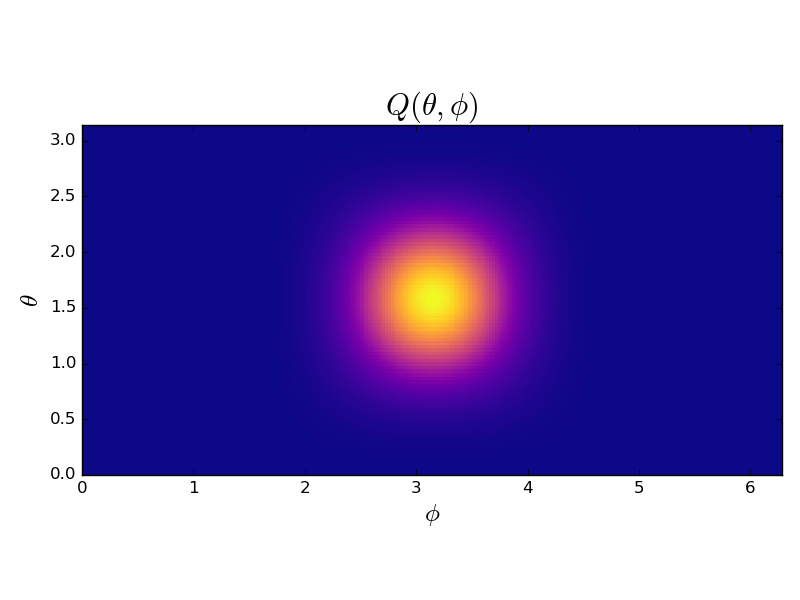
Initially, it looks like this, mirroring the isotropic nature of the variance:

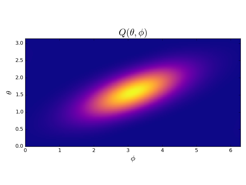
But after applying the spin squeezing operator, it looks like this:
 I.e., it is squeezed along one axis, and stretched along the perpendicular.
Quantifying Squeezing
We can quantify the degree that the state has been squeezed by comparing it to the initial state. We expect that a squeezed state should have a smaller variance in one direction than the initial state. That is, as we sweep our vector \(\hat{n}_\perp\) around the circle, we should find the angle \(\varphi\) that points in the direction where the variance of \(S_\varphi\) is smallest.
\[ \sigma^2_{\text{min}} = \min_{\varphi} \left[\left\langle S^2_\varphi \right\rangle - \left\langle S_\varphi \right\rangle^2\right] \]
To normalize this amount, we introduce the squeezing parameter, \(\xi^2\):
\[ \xi^2 = \frac{\sigma^2_{\text{min}}}{|\langle \vec{S} \rangle|^2} \]
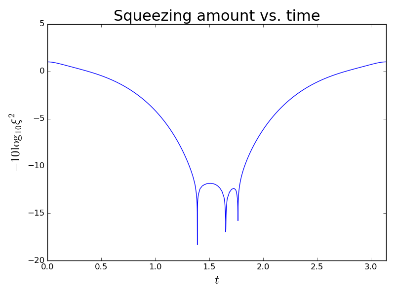
When a system is evolving under the spin squeezing operator, this quantity evolves as well:

Now in order to maximize the gains in precision by using the one-axis twisting method, we should wait until the moment \(t^*\) where \(\sigma^2_{\text{min}}(t^*)\) reaches its minimum.
\[ \xi^2_{\text{max}} = \min_t \frac{\sigma^2_{\text{min}}(t)}{\langle \vec{S} \rangle(t)} \]
This then is the maximum squeezing that we can hope to achieve. From the plot above, this happens at around \(t \approx 1.4\).
Comments