The Derivation

The equation of motion of a damped pendulum subject to a stochastic driving force is given by:

\[ X''(t) + 2\alpha X'(t) + (\omega_0^2 + \alpha^2)X(t) = W(t) \]

where \(X(t)\) is the displacement of the pendulum from its resting position, \(\alpha\) is the damping factor, and \(W(t)\) is a stochastic driving force, which may come from immersing the pendulum in a turbulent fluid.

Analytical Solution

This system can be solved analytically, and fairly quickly, so we might as well just do it. First we take the Fourier transform of both sides:

\begin{align*} \mathcal{F}(X''(t) + 2\alpha X'(t) + (\omega_0^2 + \alpha^2)X(t)) &= \mathcal{F}(W(t)) \\\
(-\omega^2 + 2i\alpha \omega + (\omega_0^2 + \alpha^2))\hat{X}(\omega) &= \hat{W}(\omega) \\\
\end{align*}

Then we solve for \(\hat{X}(\omega)\)

\begin{align*} \hat{X}(\omega) &= \frac{\hat{W}(\omega)}{(-\omega^2 + 2i\alpha \omega + (\omega_0^2 + \alpha^2))} \\\
&= -\frac{\hat{W}(\omega)}{2\omega_0} \left[ \frac{1}{(i\alpha - (\omega + \omega_0))} - \frac{1}{(i\alpha - (\omega - \omega_0))} \right] \end{align*}

and invert to get the solution:

\begin{align*} X(t) &= \mathcal{F}^{-1}(\hat{X}(\omega)) \\\
&= \frac{1}{2\pi}\int_{-\infty}^{\infty} -\frac{W(t)}{2\omega_0}\int_{-\infty}^{\infty} e^{-i\omega(t-t')}\ \left[ \frac{1}{(i\alpha - (\omega + \omega_0))} - \frac{1}{(i\alpha - (\omega - \omega_0))} \right] \mathrm{d}\omega\mathrm{d}t \end{align*}

The integral over \(\omega\) can be done via contour integration:

\begin{align*} I = \oint_\gamma e^{-i\omega (t-t')} \left[ \frac{1}{(i\alpha - (\omega + \omega_0))} - \frac{1}{(i\alpha - (\omega - \omega_0))} \right] \mathrm{d}\omega = 2\pi i\sum_{i}R_i \end{align*}

Where the contour is traversed counter-clockwise and the residues \(R_i\) are from the two poles at \(\omega = \pm \omega_0 - i\alpha\):

\begin{align*} \sum_i R_i = e^{-\alpha (t-t')}\left(e^{i\omega_0 (t-t')} + e^{-i\omega_0 (t-t')}\right) \end{align*}

So the analytical solution is:

\begin{align*} X(t) = \int_{-\infty}^{\infty}W(t')e^{-\alpha (t-t')}\frac{\sin(\omega_0 (t-t'))}{\omega_0}\mathrm{d}t' \end{align*}

which is just a convolution of \(W(t)\) with the kernel \(e^{-\alpha t}\frac{\sin(\omega_0 t)}{\omega_0}\)

Simulating with Julia

We can use the DifferentialEquations package from Julia to simulate the trajectory of this physical system.

Since we have a random component, \(W(t)\), in our equation, we will use the RODEProblem method to formulate our problem. The RODEProblem expects us to pass a first-order differential equation, so we need to rephrase the second-order DE as a pair of first-order DEs:

\begin{align*} \vec{u} &= [X, X'] \\\
\mathrm{d}u_1 &= u_2 \mathrm{d}t \\\
\mathrm{d}u_2 &= -(2\alpha u_2 + (\omega_0^2 + \alpha^2)u_1 - W)\mathrm{d}t \end{align*}

In Julia code, this is:

1
2
3
4
5
6
7
8
using DifferentialEquations
pde = function(du, u, p, t, W)
            α, ω₀ = p
            X = u[1]
            dX = u[2]
            du[1] = dX
            du[2] = -2α*dX-(ω₀² + α²)*X
      end

In order to solve this, we need to specify five things:

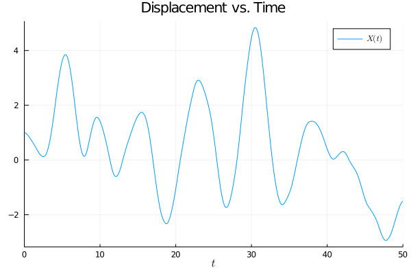
a initial condition. Here we choose \(\vec{u}(0) = [1, 0]\)
a time domain to solve this over. Here we start with \(\tau = [0, 50]\)
a solution method. We’ll use the random Euler-Maruyama algorithm RandomEM
the size of the time step. We’ll start with a moderate discretization of \(10^{-2}\)
the parameter values for \(\alpha\) and \(\omega_0\). We choose \(\alpha = 0.1\) and \(\omega_0 = 1\)

1
2
3
4
5
u_0 = [1 0]
τ = (0.0, 10.0)
p = [0.1, 0.5]
prob = RODEProblem(pde, u_0, τ, p)
sol = solve(prob, RandomEM(), dt=1/100)

We can visualize a trajectory by plotting the solution:

1
2
3
using Plots
using LaTeXStrings
plot(sol, vars=1, title="Displacement vs. Time", xaxis=L"t", label=L"X(t)")

Pendulum in a Turbulent Fluid

Analytical Solution

Simulating with Julia

Comments