In introductory statistics, you are taught that when estimating a population mean \(\mu\) and variance \(\sigma^2\) you should use the sample mean:

\[ \bar{x} = \frac{1}{n}\sum_i x_i \]

and sample variance:

\[ \widehat{\sigma^2} = \frac{1}{n-1} \sum_i \left(x_i - \bar{x}\right)^2 \]

with the hand-wavy comment that the \(n-1\) in the denominator is necessary to account for small sample sizes.

At least that was what I was told.

In this post I explain why this factor is necessary.

Everything is Random

When sampling a population, we will get a set of random values \(x_1, x_2, \dots, x_n\) which are assumed to be independent and normally distributed:

\[ x_i \sim N(\mu, \sigma^2) \]

The Sample Mean

The sample mean \(\bar{x}\) is the estimator of the population mean. From its definition:

\[ \bar{x} = \frac{1}{n}\sum_{i=1}^n x_i \]

it is then the sum of normally-distributed random variables – it too is a random variable. This means we can calculate the expectation value and the variance:

\[ E[\bar{x}] = \mu \qquad V[\bar{x}] = \frac{\sigma^2}{n} \]

Where we use the properties of the \(E\) and \(V\) functions:

\[ E[x_1 + x_2] = E[x_1] + E[x_2] \qquad V[ax_1 + ax_2] = a^2V[x_1] + a^2V[x_2] + 2a^2 \text{Cov}[x_1, x_2] \]

and the fact that the variables are assumed independent (which makes the covariance term vanish).

The Sample Variance

The population variance is defined as:

\[ \sigma^2 = \frac{1}{n}\sum_{i=1}^n(x_i - \mu)^2 \]

We usually don’t have a value for \(\mu\), so we can guess that a good estimator would be to replace \(\mu\) with \(\bar{x}\):

\[ s^2 = \frac{1}{n}\sum_{i=1}^n (x_i - \bar{x})^2 = \frac{1}{n}\sum_{i=1}^n x_i^2 - \left(\frac{1}{n}\sum_{i=1}^n x_i\right)^2 = \frac{1}{n}\left(\sum_{i=1}^n x_i^2 \right)- \bar{x}^2 \]

Now \(s^2\) is the sum of squared random variables, so it is also a random variable. If we calculate the expected value of it, we find:

\[ E[s^2] = \frac{1}{n}\sum_{j=1}^n s^2 \]

\[ = E\left[\frac{1}{n}\left(\sum_{i=1}^n x_i^2 \right)- \bar{x}^2\right] = \frac{1}{n}\sum_{i=1}^n E\left[x_i^2\right] - E\left[\bar{x}^2\right] \]

This expression involves evaluating the expectation of the square of normally-distributed random variables. To evaluate each of these terms, we can employ the value of the second moment of the normal distribution:

\[ E[z^2] = \frac{1}{\sqrt{2\pi} w}\int_{-\infty}^{\infty} \exp{\left(\frac{z - m}{w}\right)^2}z^2 \mathrm{d}z = m^2 + w^2 \]

If \(x_i \sim N(\mu, \sigma^2)\), the first term is \(\mu^2 + \sigma^2\). If \(\bar{x} \sim N(\mu, \frac{\sigma^2}{n})\), the second term is \(\mu^2 + \frac{\sigma^2}{n}\). Putting it together, we have:

\[ E[s^2] = \left( \mu^2 + \sigma^2 \right) - \left( \mu^2 + \frac{\sigma^2}{n} \right) = \sigma^2 - \frac{\sigma^2}{n} = \frac{n-1}{n}\sigma^2 \]

Bias in the Estimator

Now that we know the expected value of our estimator, we turn to the definition of bias in an estimator. The bias, \(b\), in an estimator \(\hat{\theta}\) of a parameter \(\theta\) is the difference between the expected value of the estimator and the value of the parameter estimated:

\[ b(\hat{\theta}) = E[\hat{\theta}] - \theta \]

In the case of the sample variance, the estimated value is the variance of the population, \(\sigma^2\). So the bias would be:

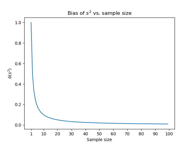
\[ b(s^2) = E[s^2] - \sigma^2 = \frac{n-1}{n}\sigma^2 - \sigma^2 = \frac{1}{n}\sigma^2 \]

Below is a plot of \(b(s^2)\) as a function of \(n\).

 1
 2
 3
 4
 5
 6
 7
 8
 9
10
11
12
13
14
15

import matplotlib.pyplot as plt
import numpy as np

x = np.arange(1,100)
y = 1.0/x

fig, ax = plt.subplots()

ax.plot(x, y)
ax.set_title('Bias of $s^2$ vs. sample size')
ax.set_xlabel('Sample size')
ax.set_xticks([1, *np.arange(10,101,10).tolist()])
ax.set_xticklabels([1, *np.arange(10,101,10).tolist()])
ax.set_ylabel('$b(s^2)$')

As we were promised, it is only large for small values of \(n\). But since it is always positive, our estimator \(s^2\) will always be larger than the true value of \(\sigma^2\).

Fixing the Bias

In order to account for the bias in our estimator, let us define a new estimator \(\hat{\sigma^2}\):

\[ \widehat{\sigma^2} = \frac{n}{n-1}s^2 = \frac{1}{n-1}\sum_{i=1}^n \left(x_i - \bar{x}\right)^2 \]

Now we can check (using the fact that \(E[ax] = aE[x]\)) that the bias of this estimator is zero for all \(n\). Therefore we use \(\widehat{\sigma^2}\) as the sample variance instead of the naive estimator \(s^2\). \(\blacksquare\)