Using autograd in Python for Quantum Computing
I recently participated in a challenge in quantum computing posed by the Quantum Open Source Foundation. In this post, I recap the problem description and my solution to the challenge. The challenge involves exploring the ability of a certain class of quantum circuits in preparing a desired four-qubit quantum state. In this challenge, the problem is to optimize a quantum circuit composed of layers of parameterized gates. To solve this, we implement the circuit in Python and optimize the parameters using the autograd library.
Goal
The cost function we are going to minimize is:
\[ \varepsilon = \min_{\theta}\left||\psi(\theta)\rangle - |\phi\rangle \right| \]
where \(|\psi(\theta)\rangle\) is the state of the system after going through the circuit and the initial state is \(|\psi\rangle = |0000\rangle\).
We choose the state \(|\phi\rangle\) to be the 4-qubit GHZ state:
\[ \left|\phi\right\rangle = \frac{1}{\sqrt{2}} \left(\left|1111\right\rangle + \left|0000\right\rangle\right) \]
Circuit Description
The circuit is composed of a variable number of layers of blocks. There are only two types of blocks — odd and even — and they have parameters we can tweak to prepare the given state. The blocks are arranged QAOA-style, which means each layer has the even block following the odd block.
The even blocks are composed of the following gates:
In mathematical notation:
\[ U_i^{\text{even}}(\theta_{i,n}) = \left(\prod_{\langle j,k \rangle}CZ(j,k) \bigotimes_{n=1}^4 R_{z}(\theta_{i,n}) \right) \]
The odd blocks are composed of the rotation-X gates:
In mathematical notation:
\[ U_i^{\text{odd}}(\theta_{i,n}) = \left( \bigotimes_{n=1}^{4} R_{x}(\theta_{i,n}) \right) \]
The operator for the \(\ell^{\text{th}}\) layer is:
\[ U_{\ell} = U^{\text{even}}_{2\ell} U^{\text{odd}}_{\ell} \]
Implementation
In the Python code below, we calculate \(\varepsilon\) by constructing the unitary operator for the circuit with a specified number of layers (n_layers), and then we use the autograd library to find the minimum.
But first we have define our gates:
| |
From these basic gates we can create the blocks:
| |
And from the blocks, we can create the layers:
| |
and define the circuit:
| |
To setup the minimization, we need to specify an objective function (i.e. \(\varepsilon\)) to auto-differentiate.
The following code block loads the autograd library, encodes our cost function in the objective function and computes the AD gradient.
| |
To implement the minimization, we need to specify a few things:
- a minimizer (here we choose
adam) - the initial values for the parameters \(\theta_{i,n}\): I use samples from the normal distribution \(N(0,\pi^2)\)
- the step size and the number of iterations: I chose a step size of 0.1 and at least 400 iterations. The trade-off here is speed vs. accuracy.
We call the minimizer by passing these configuration options to adam. It will return us the optimized values for \(\theta_{i,n}\), which we then use to compute \(\varepsilon\) by passing them to the objective function.
| |
For debugging purposes, we also pass a callback to our minimization routine – here’s the definition of handle_step, which prints the objective every 20 steps:
| |
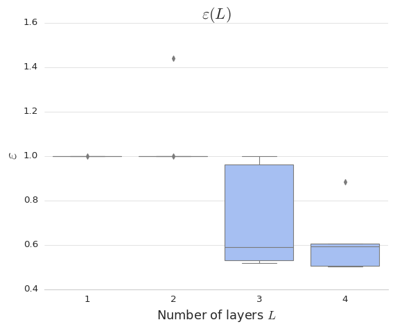
After running this with over a few layers and iterations, we can check the optimal value of our cost function \(\varepsilon\) via a plot.
In the figure below, we have plotted the ranges of values of \(\varepsilon\) that the adam optimizer returns, for one, two, three, and four layers respectively.
Since we are using a stochastic algorithm, the results are not the same every time, so we use a boxplot to see the distribution of results for each layer.

Sanity check: does the range of values for \(\varepsilon\) make sense?
Well, our cost function involves the magnitude of the difference of two normalized vectors. The maximum difference of two normalized vectors is 2, when they are pointing in exactly opposite directions. The minimum difference would be 0, when they are perfectly aligned. Since the plot shows results between 0.4 and 1.6, we can conclude that the results are not totally out-of-the-question.
From this plot, we can see that, for a small number of layers, more layers yields a better result.
This means that we can take the results of the optimization for n_layers = 4, and plug them into our quantum circuit, and approximate the GHZ state!
Comments