Principal component analysis, or PCA, is used to characterize a highly multi-dimensional data set in terms of its main sources of variation. It is a dimensionality-reduction technique, which helps to avoid the curse of dimensionality. Here’s the main idea:

Let’s say we have a \(n\) - dimensional distribution with random variables \(X_1, X_2, \dots, X_n\). We can take these variables to be uncorrelated, with mean zero, without loss of generality. If we take \(N\) samples for each variable in this distribution, we can calculate the set of sample variances:

\[ \widehat{\sigma^2_{x_i}} = \frac{1}{N-1}\sum_{j=1}^N x_{ij}^2 - \bar{x_i}^2 \]

Let’s say we find that among the variables, \(x_3\) has the smallest variance. In the limit that the variance for \(x_3\) is zero (\(\widehat{\sigma^2_{x_3}} = 0\)), there is no variation in the \(X_3\) variable. In this case, we could remove the variable from our sample set, and our models would perform just as well. If we did this, the data set effectively becomes \((n-1)\) -dimensional. Generalizing, if we have \(k\) variables with sample variance zero, we could remove those as well, making our data set \((n-k)\) -dimensional.

Usually, we don’t find that the sample variance is zero in any of our variables, so we approximate by removing the variable(s) with the least variance. The remaining variable(s) are called the principal components.

There are complications when there are correlations between the variables – but this can also be accounted for.

Adding Correlations

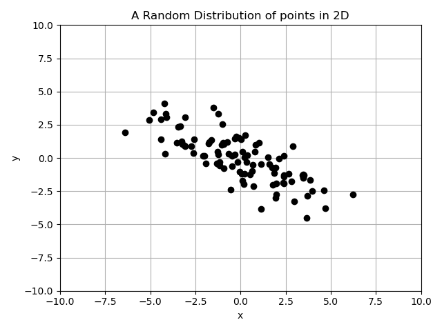
Here’s a 2-dimensional data set with correlations to illustrate how this can get complicated:

If we calculate the sample variance of each of the variables as:

$$\widehat{\sigma^2_x} = 6.57, \qquad \widehat{\sigma^2_y} = 3.51$$

It looks like the variable with the lowest variance is the \(y\) variable. But there is a slight negative correlation between \(x\) and \(y\) in this data set. In fact, if we calculate the sample variance along the direction of \(\vec{e}_1 = \frac{1}{\sqrt2} \hat{i} + \frac{1}{\sqrt2} \hat{j}\):

\[ \widehat{\sigma^2_{\vec{x}\cdot\vec{e}_1}} = \frac{1}{2}\widehat{\sigma^2_x} + \frac{1}{2}\widehat{\sigma^2_y} + \widehat{\text{Cov}}(x,y) \]

We find that

$$\widehat{\sigma^2_{\vec{x}\cdot\vec{e}_1}} = 3.24$$

Note that \[ \widehat{\sigma^2_{\vec{x}\cdot\vec{e}_1}} < \widehat{\sigma^2_y} \]

Therefore, when the variables are correlated, a linear combination of variables may have less variance than any individual variable. In our example, we can define \(y' = \frac{1}{\sqrt{2}}x + \frac{1}{\sqrt{2}}y\) as a factor in a new 2D model, which has variables \((x', y')\). To define \(x'\), we can form a vector perpendicular to \(\vec{e}_1\), that is, the vector \(\vec{e}_2 = -\frac{1}{\sqrt{2}}\hat{i} + \frac{1}{\sqrt{2}}\hat{j}\). Calculating the variance along this vector, we find:

$$\widehat{\sigma^2_{\vec{x}\cdot\vec{e}_2}} = 10.3$$

And note that:

\[ \widehat{\sigma^2_{\vec{x}\cdot\vec{e}_2}} > \widehat{\sigma^2_x} \]

So \(\vec{e}_2\) captures more of the variance than the \(x\) variable by itself.

Therefore, in the transformed 2D data set, \(x'\) would be the principal component, and we would remove \(y'\) from our models.

Generalizing

We can generalize this by parameterizing the vectors in terms of a dummy variable \(\theta\):

\[ \vec{e_1} = \cos(\theta)\hat{i} +\sin(\theta)\hat{j} \]

\[ \vec{e_2} = \sin(\theta)\hat{i} - \cos(\theta)\hat{j} \]

The expression for the sample variance is then:

\begin{equation} \widehat{\sigma^2_{\vec{x}\cdot\vec{e_1}}} = \cos^2(\theta)\widehat{\sigma_x^2} + \sin^2(\theta)\widehat{\sigma^2_y} + \sin(2\theta)\widehat{\text{Cov}}(x,y) \label{eq:1} \end{equation}

We can find the components by maximizing this expression with respect to \(\theta\):

\[ \theta^{*} = \text{arg}\max_\theta \widehat{\sigma^2_{\vec{x}\cdot\vec{e_1}}} \]

Since this example is in 2D, we only have to find one parameter. But in \(d\) -dimensions, we would need \((d-1)\) parameters. This process is obviously not efficient. So let’s find a better way.

Inspiration from Geometry

If you squint, the expression we tried to maximize in \eqref{eq:1} looks like the equation for an ellipse:

\[ 0 = a x^2 + c y^2 + 2bxy \]

and if we remember our geometry, the principal axes of such an ellipse can be derived from the eigenvectors of the corresponding matrix:

\[ A = \begin{pmatrix} a & b \\ b & c \end{pmatrix} \]

Further, this method works for \(n\) -dimensional ellipsoids. Therefore, if we could make the correspondence exact, the problem of finding the vectors \(\vec{e_1}, \vec{e_2}, \dots, \vec{e_n}\) could be reduced to finding the eigenvectors of a specific matrix.

Fortunately, we have such a matrix readily available: consider rewriting \eqref{eq:1} as:

\[ \widehat{\sigma^2_{\vec{x}\cdot\vec{e_1}}} = \vec{e_1}^T M \vec{e_1} \]

\[ \vec{e_1} = \begin{pmatrix} \cos\theta & \sin\theta \end{pmatrix} \] \[ M = \begin{pmatrix} \widehat{\sigma_x^2} & \widehat{\text{Cov}}(x,y) \\ \widehat{\text{Cov}}(y,x) & \widehat{\sigma_y^2} \end{pmatrix} \]

\(M\) is just the sample covariance matrix. Therefore, in order to find the principal components for any dimensional data set, we will use the eigenvectors of the sample covariance matrix. Once we have calculated them, we can identify the components with the least variance, and remove them.

Conclusion

We can summarize the above into the following algorithm:

1. Calculate the sample covariance matrix
2. Find the eigenvectors of said matrix
3. Remove (or ignore) the components which have the least variance

What you end up with is a smaller-dimensional data set, while still capturing most of the variation in the data. The components then can be used for model building, but that is a subject for a different post.