Noisy-OR model in Bayesian Networks
A common application of IoT sensors is for alerting of the presence of a specific event – be it a leaking appliance, a broken piece of equipment, or a home invasion (i.e. burglar alarm). Due to the imperfect nature of these sensors, and the random, unpredictable world they live in, detecting a specific event cannot be done perfectly. Instead, we can only infer the presence of some event with some “noise”, or uncertainty.
Bayesian networks offer a framework for inferring the presence of an event from the detection data on a sensor, while allowing for this uncertainty.
In this post we explore a specific network – the noisy-OR model – as a starting point for accommodating uncertainty when inferring the presence of a specific event in the midst of other possible causes of the alert. I also offer an example application of the model to a real-world scenario.
Background
The Noisy-OR Bayesian network requires specifying three items:
- The set of events to be detected.
- The prior probability that each event will occur.
- The probability that each event will go undetected.
We model the set of events that can occur as a set of boolean random variables. Note – it is essential that the events are independent, and no causal link exists between them. Let \(X = \{x_i\}_{i=1}^N\) be a set of boolean random variables, \(x_i \in \{0,1\}\). Then \(x_i=1\) indicates that the \(i^{th}\) event has occurred; the value of \(\Pr[x_i=1]\) denotes the prior probability that event \(x_i\) will occur.
We can model the uncertainty as a set of functions that randomly negate the value of each \(x_i\): let \(F = \{f_i\}_{i=1}^N\) be a set of functions \(f_i: x_i \mapsto x_i'\), where \(x_i\) represents the \(i^{th}\) event occuring, but \(x_i'\) represents whether the sensor actually detected the the \(i^{th}\) event. Then, the probability of the sensor detecting the \(i^{th}\) event (or not), given that the \(i^{th}\) event occurred (\(x_i=1\)) or not (\(x_i=0\)) is specified by the table:
\begin{array}{cc|c}
x_i & x_i' & \Pr[x_i' | x_i] \\ \hline
0 & 0 & 1 \\
0 & 1 & 0 \\
1 & 0 & q_i \\
1 & 1 & 1-q_i \\
\end{array}
These functions represent the imperfection of the sensor in detecting each of the events. When a event occurs (\(x_i = 1\)), there is a probability \(q_i\) that it will not be detected. The \(f_i\) can also be defined graphically as:
Now, if any of the detectable events are detected, the sensor will necessarily alert. Therefore, let \(g\) be the logical OR function over the set \(\{x_i'\}_{i=1}^N\):
\begin{equation*} g = \bigvee_{i=1}^N x_i' \end{equation*}
If \(g=1\), then that implies the sensor has detected at least one event; if \(g=0\), then the sensor has not detected an event.
Putting these definitions together, we have a Bayesian network that can be represented graphically as:
The probability of any state of this network is captured by the joint distribution \(\Pr[g, X', X]\). Thanks to the network structure, we can factorize this joint distribution as:
\begin{equation} \Pr[g,X',X] = \Pr[g|X]\Pr[X] \label{eq:1} \end{equation}
To compute the distribution \(\Pr[g,X',X]\) of this network, first consider the probability of \(g=0\). The only way to obtain \(g=0\) is if all the \(x_i'\) s are zero. This follows from the defintion of the logical OR operation:
\begin{equation*} \left(\bigvee_{i=1}^N x_i'\right) = 0 \implies \bigwedge_{i=1}^N(x_i' = 0) \end{equation*}
Therefore, in \eqref{eq:1}, we can replace \(g=0\) with the result:
\begin{equation*} \Pr[g=0|X] = \Pr\left[\left.\bigwedge_{i=1}^N x_i' = 0 \right| X\right] = \prod_{i=1}^N \Pr[x_i' = 0 |X] \end{equation*}
By looking at the table, we can see that each \(x_i'\) can be zero, given \(X\), in one of two ways:
- The corresponding \(x_i\) is identically zero
- The corresponding \(x_i\) was 1, but the \(f_i\) flipped it: \(f_i(x_i) = 0\). This occurs with probability \(q_i\).
If we have \(j\) values of \(x_i\) falling into the second category, and the rest identically zero, then we have:
\begin{align*}
\Pr[g=0| X] &= \Pr[g=0|\{x_1=1, \dots, x_j=1, x_{j+1}=0, \dots, x_N=0\}] \\\
&= \prod_{i=1}^j \Pr[x_i'=0|x_i=1] \prod_{i=j}^N \Pr[x_i'=0|x_i=0] \\\
&= \prod_{i=1}^j q_i \prod_{i=j}^N (1) \\\
&= \prod_{i=1}^j q_i
\end{align*}
The remaining probability \(\Pr[g=1|X]\) is just \(1-\Pr[g=0|X]\)
\begin{equation} \Pr[g=1|X] = 1 - \prod_{i=1}^j q_i \label{eq:2} \end{equation}
We can re-write this slightly to allow the \(x_i\) to appear in any order: let \(I_1 = \{i | x_i = 1\}\) be the index set of the \(x_i\) which are equal to 1. Then:
\begin{align*}
\Pr[g=0|X] &= \prod_{i \in I_1} q_i \\\
\Pr[g=1|X] &= 1-\prod_{i \in I_1} q_i
\end{align*}
With this, and the specification of the prior probabilities \(\Pr[x_i]\), we have completely enumerated the probabilities of the sensor detecting any of the events.
Application: Inference
The specification of the probability \(\Pr[g,X',X]\) can be applied to quantifying the uncertainty that comes with the detection of an event. Returning to our original motivation, we can now pose the question of detecting the specific event in the presence of “noise”.
Question: If we let \(x_{j}=1\) indicate the presence of the specific event we care about, and the other \(\{x_i\}_{i\neq j}\) be “noise”, then what is the probability that the \(j^{th}\) event has occurred, given that the sensor has told us that it has detected an event (\(g=1\))? In other words, what is \(\Pr[x_j=1|g=1]\)?
To answer this question, we use Bayes' Theorem:
\begin{equation*} \Pr[x_j=1|g=1] = \frac{\Pr[g=1|x_j=1]\Pr[x_j=1]}{\Pr[g=1]} \end{equation*}
The first term in the numerator is just \eqref{eq:2}, summed over the “noise” events. Therefore, let’s define \(X^* = \{x_i\}_{i\neq j}\) as the set of “noise” events, so we can write this term as:
\begin{align*}
\Pr[g=1|x_j=1] &= \sum_{x_i \in X^*}\Pr[g=1, X^* | x_j=1]\\\
&= \sum_{x_i \in X^*} \Pr[g=1,|x_j=1, X^*]\Pr[X^*] \\\
&= \sum_{x_i \in X^*} \left[\left(1-q_j \prod_{i \in I_1}q_i\right) \prod_{i\neq j} \Pr[x_i] \right]
\end{align*}
The term in the denominator is:
\begin{align*}
&\Pr[g=1] = \sum_{x_i \in X} \Pr[g=1,X] \\\
&= \sum_{x_i \in X^*} \Pr[g=1|x_j=1]\Pr[x_j=1] + \Pr[g=1|x_j=0]\Pr[x_j=0] \\\
\end{align*}
The first term in the sum is:
\begin{equation*} \sum_{x_i \in X^*} \left[\left(1-q_j \prod_{i \in I_1}q_i\right) \prod_{i\neq j} \Pr[x_i]\right]\Pr[x_j=1] \end{equation*}
The second term is like it:
\begin{equation*} \sum_{x_i \in X^*} \left[\left(1- \prod_{i \in I_1}q_i\right) \prod_{i\neq j} \Pr[x_i]\right]\Pr[x_j=0] \end{equation*}
With that, we have answered the original question, in terms of the various parameters that might differ from one situation to the next. We can apply these formula to a concrete example by specifying the prior probabilities \(\Pr[x_i]\) and the conditional probabilities of detection \(\Pr[x_i'=1|x_i=1] = 1-q_i\).
Example
Let’s say we have a smoke detector that will alarm in the presence of fire, cigarette smoke, or due to a internal component failure. Let’s say the prior probabilities of each event are:
- Fire: \(\Pr[x_1=1] = 0.001\)
- Cigarette Smoke: \(\Pr[x_2=1] = 0.05\)
- Internal failure: \(\Pr[x_3=1] = 0.0001\)
The conditional detection probability of the smoke detector is:
- Fire: \(\Pr[x_1'=1|x_1=1] = 1-0.001 = 0.999\). \((q_1 = 0.001)\)
- Cigarette Smoke: \(\Pr[x_2'=1|x_2=1] = 1-0.01 = 0.09\). \((q_2 = 0.01)\)
- Internal failure: \(\Pr[x_3'=1|x_3=1] = 1-0.05 = 0.95\). \((q_3 = 0.05)\)
We are interested in finding the probability that there is a fire, given an alarm. This is the value of \(\Pr[x_1=1|g=1]\). We can compute it by applying the formula from the previous section. To expedite the calculations, we can use a short Python script to do it for us:
| |
The result of the calculation is 0.0198. That is, we only have a small chance that an actual fire has happened, given the alarm. Considering the other possible causes, this should be a relief!
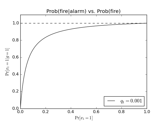
We can look at the behavior of this value as a function of the prior probability \(\Pr[x_1=1]\) that a fire has occurred:

We can see that the probability saturates quite quickly as the prior probability increases. Alternatively, we can consider varying the detection reliability:

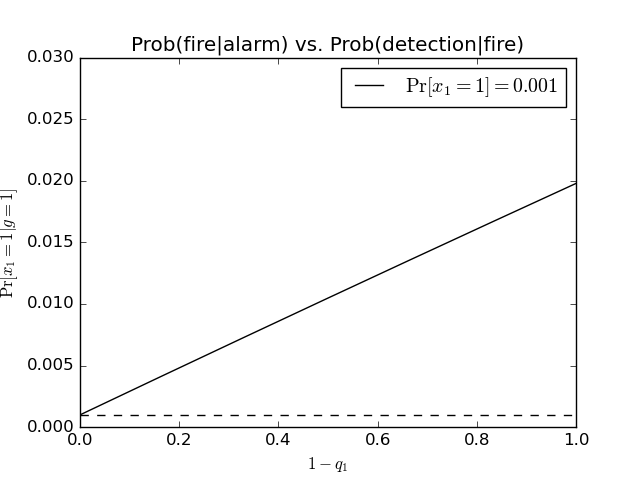
The dotted line is a horizontal line at \(0.001\) – the value of the prior \(\Pr[x_1=1]\). The two lines intersect at \(1-q_1 = 0\) (i.e. the sensor is completely unable to detect smoke reliably). This makes sense – in the limit that the detection reliability is zero, then hearing the alarm doesn’t increase the likelihood that there is a fire at all.
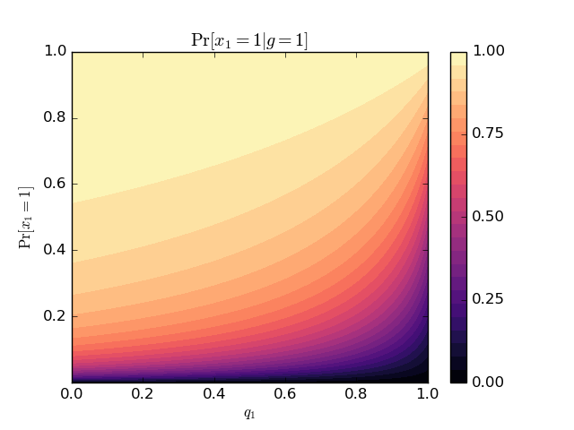
Finally, if you’re still interested, I plotted the posterior as a function of the prior and detection reliability:

Comments