Most of us have heard the story of “the boy who cried wolf”. A town’s herald boy is charged with alerting the town of the presence of a wolf. However, he has a proclivity for lying, and because of this, his alerts are unreliable. Eventually, the townsfolk have a difficult time inferring the presence of wolf from the boy’s reports.

Though this story is simple, it is a perfect case to illustrate the application of Bayesian inference. This method are frequently employed to solve problems in artificial intelligence applications, but is probably the most intuitive mathematics I have seen.

Inference: Logical and Bayesian

There are multiple ways that we can infer something from something else. One of these is logical inference, evident in the syllogism:

1. If it is raining outside, then the streets are wet
2. It is raining outside
3. Therefore the streets are wet

Another is Bayesian inference, also called abduction, which is inference to the best explanation, on the grounds of the evidence. It is an admittedly weaker form of inference, but sometimes that’s the best we can do. An example of this type of inference would be:

1. If it is raining outside, then the streets are wet
2. The streets are wet
3. Therefore it is probably raining

Bayesian inference gives us a mathematical framework to quantify the probability in (3), if we provide the data for (2). The basic tool is conditional probability, which leads to Bayes' rule

Conditional Probability and Bayes' Rule

For the purposes of this post, we will define the conditional probability \(P(a|b)\) that the event \(a\) occurs, given that \(b\) occurs, in terms of the joint probability distribution:

\(P(a|b) = P(a,b)/P(b)\)

where \(P(b) = \sum_a P(a,b) = \sum_a P(b|a)P(a)\)

From this definition follows Bayes Rule:

\begin{align*} P(a|b)P(b) &= P(b|a)P(a) \\\
\implies P(a|b) &= \frac{P(b|a)P(a)}{P(b)} \end{align*}

Bayes' rule allows us to compute the probability of a cause, given one of its effects. To illustrate, let’s return to the story of the boy who cried wolf. Let \(a \in \{0,1\}\) indicate the absence or presence of a wolf. Let \(b \in \{0,1\}\) indicate the absence or presence of the boy’s alert. From here, we can pose the question on everyone’s mind when the boy alerts of a wolf: what is the probability that there is a wolf \((a=1)\), given the boy’s alert \((b=1)\)?

That is, we seek \(P(a=1|b=1)\). Using Bayes rule, this is:

\begin{equation*} P(a=1|b=1) = \frac{P(b=1|a=1)P(a=1)}{P(b=1)} \end{equation*}

The three terms we need to evaluate are:

1. \(P(b=1|a=1)\): Likelihood that the boy alerts the townsfolk, given the presence of a wolf
2. \(P(a=1)\): Probability that a wolf is present, whether or not we get an alert
3. \(P(b=1)\): Probability that the boy alerts the townsfolk, whether or not there is a wolf

In this representation of the story, the boy always alerts when the wolf is present, so \(P(b=1|a=1) = 1\).

The factor \(P(a=1)\) requires prior information to quantify – let’s say the town’s wolf expert has long been keeping track of wolf encroachment on the town, and knows that during this time of year, a wolf encounter occurs about once a month, so \(P(a=1) = 1/30\)¹.

The factor in the denominator \(P(b=1)\) can be expanded out as:

\begin{align*} P(b=1) &= \sum_{a \in \{0,1\}} P(b=1|a)P(a) \\\
&= P(b=1|a=1)P(a=1) + P(b=1|a=0)P(a=0) \\\
&= \left[P(b=1|a=1) - P(b=1|a=0)\right]P(a=1) + P(b=1|a=0) \\\
&= \frac{1}{30}(1-P(b=1|a=0)) + P(b=1|a=0) \\\
\end{align*}

From here, we only need to specify \(P(b=1|a=0)\), which is the probability that the boy is lying. Let’s call this \(f\)

Putting it all together, we have:

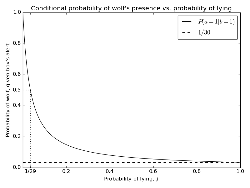
\begin{equation*} P(a=1|b=1) = \frac{\frac{1}{30}}{(1-f)\frac{1}{30} + f} = \frac{1}{1+29f} \end{equation*}

Sanity check: what happens when the boy never lies \((f=0)\), or when he always lies \((f=1)\)?

\begin{equation*} P(a=1|b=1) = \begin{cases} 1 & f = 0 \\\
1/30 & f = 1 \end{cases} \end{equation*}

This makes sense – it tells us that if the boy never lies, we can infer the presence of the wolf with certainty. On the other hand, if he always lies, then we can only infer the presence of the wolf up to the probability specified by the expert, i.e., with probability \(1/30\).

Going back to the original story, we see that after hearing the boy’s alert, the townsfolk have to make a decision – to either take evasive action or ignore the boy’s plea. Assuming their tolerance for risk is balanced, it would make sense for them to hide if they think \(P(a=1|b=1) > 0.5\), and ignore the message if \(P(a=1|b=1) < 0.5\). In this case, we can see just how damaging the boy’s lying is from the plot – people will ignore him if they think he lies more often than once every 29 alerts. This is exactly what happens in the story.

Conclusion

In this brief introduction to Bayesian inference, we have already seen how Bayes' rule is central to problems in probabilistic inference. In the example, we see how to model the task of inferring the presence of an uncertain cause, given an somewhat unreliable effect. Though it may seem simplistic, this situation and its generalizations will show up throughout probabilistic inference, and I hope to illustrate in an upcoming post how to do this.